Plotting Bézier curves directly and with De Casteljau's algorithm

Last major Update: 21.10.2013

Github repo that contains the presented code in this post.

Introduction

In this article I will present you a very simple and in no sense optimized algorithm written in Python 3 that plots quadratic and cubic Bézier curves. I'll implement several variants of Bézier rasterization algorithms. Let's call the first version the direct approach, since it computes the corresponding x and y coordinates directly by evaluation of the equation that describes such Bézier curvatures.

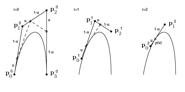
The other possibility is De Casteljau's algorithm, a recursive implementation. The general principle is illustrated here. But the summarize the idea very briefly: In order to compute the points of the Bézier curve, you subdivide the lines of the outer hull that are given from the n+1 control points [Where n denotes the dimension of the Bézier curve) at a ratio t (t goes from 0 to 1 in a loop). If you connect the interpolation points, you'll obtain n-1 connected lines. Then you apply the exactly same principle to these newly obtained lines as before (recursive step), until you finally get one line remaining. Consider again the point at the ratio t on this single line left and BOOM you got your point on the Bézier curve for your specific t value. Increase t and continue this process until you plotted the curve (Graphic equivalent of the description see below. I don't own the image, the source is: http://wiki.ece.cmu.edu)
Casteljau
Principle
In this article, I'll supply source code snippets for both algorithms mentioned above and will add a simple performance test to compare them. Additionally, I am going to polish the direct approach for performance and will depict some recipes I learned from other blogs to increase the efficiency of the plotting algorithm.

Background. Splines, What for?

But why do I even need such geometrical primitives? I am currently working on my captcha wordpress plugin, which builds the captcha from the ground up and therefore needs some mechanism to rasterize geometrical figures such as characters (Yes for once I am talking of those, not the data type\^\^). Thus I need three different shapes: Simple lines, circles (or more generally ellipses) and lastly Bézier curves. I could compose rudimentary characters just with lines and circles but we do have some ambition over here, don't we? :)

This means that I will essentially define a new, but very primitive font. I guess that my font will contain around 10 to 15 glyphs and it will use a mezcla (mix) of bitmap and outline fonts techniques. If you want to know more about them, just read it up . I am also going to publish a separate post blog about this font project in the near future, so stay tuned (Edit: The future has arrived. I am really excited about how ugly and cruel this font is going to be (Actually that's even an advantage for CAPTCHAS).

If you are further interested in the technical background knowledge and mathematical properties of Bézier splines, consider reading the Wikipedia article or this wonderful tutorial and then there's also this nice introduction. The authors of those articles explain the concepts ways better than a layman as I ever could. Here, I just present some simple code snippets to get started and wet the appetite, as well as a discussion of performance issues.

Finally we get to see some actual code. This python script essentially draws quadratic and cubic Bézier curves. That's the direct approach as stated above. Note that the code is yet horribly unoptimized.

import tkinter
import math

class Bezier(tkinter.Canvas):
    '''
    Simple and slow algorithm to draw quadratic and 
    cubic Bézier curves. Heavily inspired by http://pomax.github.io/bezierinfo/#control
    This code should just prove a concept and is not intended to be 
    used in a real world app...
    Author: Nikolai Tschacher
    Date: 07.10.2013
    '''
    # Because Canvas doesn't support simple pixel plotting,
    # we need to help us out with a line with length 1 in
    # positive x direction.
    def plot_pixel(self, x0, y0):
        self.create_line(x0, y0, x0+1, y0)

    # Calculates the quadtratic Bézier polynomial for 
    # the n+1=3 coordinates.
    def quadratic_bezier_sum(self, t, w):
        t2 = t * t 
        mt = 1-t
        mt2 = mt * mt
        return w[0]*mt2 + w[1]*2*mt*t + w[2]*t2

    # Calculates the cubic Bézier polynomial for 
    # the n+1=4 coordinates.
    def cubic_bezier_sum(self, t, w):
        t2 = t * t
        t3 = t2 * t
        mt = 1-t
        mt2 = mt * mt
        mt3 = mt2 * mt
        return w[0]*mt3 + 3*w[1]*mt2*t + 3*w[2]*mt*t2 + w[3]*t3

    def draw_quadratic_bez(self, p1, p2, p3):
        t = 0
        while (t < 1):
            x = self.quadratic_bezier_sum(t, (p1[0], p2[0], p3[0]))
            y = self.quadratic_bezier_sum(t, (p1[1], p2[1], p3[1]))
            # self.plot_pixel(math.floor(x), math.floor(y))
            self.plot_pixel(x, y)
            t += 0.001 # 1000 iterations. If you want the curve to be really
                       # fine grained, consider "t += 0.0001" for ten thousand iterations.

    def draw_cubic_bez(self, p1, p2, p3, p4):
        t = 0
        while (t < 1):
            x = self.cubic_bezier_sum(t, (p1[0], p2[0], p3[0], p4[0]))
            y = self.cubic_bezier_sum(t, (p1[1], p2[1], p3[1], p4[1]))
            self.plot_pixel(math.floor(x), math.floor(y))
            t += 0.001


if __name__ == '__main__':
    master = tkinter.Tk()
    w = Bezier(master, width=1000, height=1000)
    w.pack()

    # Finally draw some Bézier curves :)
    #w.draw_quadratic_bez((70, 250), (62, 59), (250, 61))
    #w.draw_quadratic_bez((170,77), (162, 159), (210, 161))
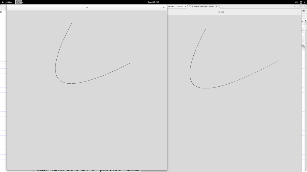
    w.draw_quadratic_bez((0, 100), (162, 89), (250, 61))
    #w.draw_cubic_bez((120, 160), (35, 200), (153, 268), (165, 70))
    tkinter.mainloop()

And now De Casteljau’s algorithm. It's not limited to quadratic and cubic Bézier curves, on the contrary, you are free to plot curves of any degree n. Just give it a try!

import tkinter

class InvalidInputError(Exception):
    pass

class Casteljau(tkinter.Canvas):
    '''
    Implementation of de Casteljau's algorithm for drawing Bézier curves.
    Implemented along the submittal of http://pomax.github.io/bezierinfo/#control.
    Author: Nikolai Tschacher
    Date: 07.10.2013
    '''
    # Because Canvas doesn't support simple pixel plotting,
    # we need to help us out with a line with length 1 in
    # positive x direction.
    def plot_pixel(self, x0, y0):
        self.create_line(x0, y0, x0+1, y0)

    def draw_curve(self, points, t):
        # Check that input parameters are valid. We don't check wheter 
        # the elements in the tuples are of type int or float.
        for p in points:
            if (not isinstance(p, tuple) or not len(p) == 2):
                raise InvalidInputError('points is not a list of points(tuples)')
        if (len(points) == 1):
            self.plot_pixel(points[0][0], points[0][1])
        else:
            newpoints = []
            for i in range(0, len(points)-1):
                x = (1-t) * points[i][0] + t * points[i+1][0]
                y = (1-t) * points[i][1] + t * points[i+1][1]
                newpoints.append((x, y))
            self.draw_curve(newpoints, t)

    # Use De Casteljau's algorithm with recursion eliminated, but the same
    # geometrical approach. Idea: Eliminate the expensive stack frame generation
    # that recursion comes with. Only quadratical Bézier curves.
    def draw_point2(self, points, t):
        # Vector addition of P0+P1
        q0_x, q0_y = ((1-t) * points[0][0] + t * points[1][0],
                        (1-t) * points[0][1] + t * points[1][1])
        q1_x, q1_y = ((1-t) * points[1][0] + t * points[2][0],
                        (1-t) * points[1][1] + t * points[2][1])

        b_x, b_y = ((1-t)*q0_x + t*q1_x, (1-t)*q0_y + t*q1_y)
        self.plot_pixel(b_x, b_y)

    # Usage function for the algorithm.
    def draw(self, points):
        t = 0
        while (t <= 1):
            self.draw_curve(points, t)
            t += 0.001

if __name__ == '__main__':
    master = tkinter.Tk()
    w = Casteljau(master, width=1000, height=1000)
    w.pack()

    # Finally draw some Bézier curves :)
    w.draw([(70, 250), (462, 159), (0, 0)])
    #w.draw([(133, 267), (121, 28), (198, 270), (210, 29)])
    tkinter.mainloop()

And finally the performance comparison between the two algorithms. The direct approach wins over De Casteljau’s algorithm (I guess because recursion is such a slowpoke), but on the other side, De Casteljau's method is numerically stable. The direct approach is a little more than twice as fast (This might not be accurate, since Python isn't really the language you use for such stuff and additionally my implementation is certainly not good enough such that I can say that any De Casteljau algorithm implementation is exactly twice as slow as the direct approach. These comparisons are rather a rough estimation)! Note that the initial type checks in draw_curve() in class Casteljau were disabled while testing the speed to avoid contortions. Furthermore, I've shamelessly stolen the timing method from this site, using the following little class to time within with statements:

import time

class Timer(object):
    def __init__(self, msg='', verbose=True):
        self.verbose = verbose
        self.msg = msg

    def __enter__(self):
        self.start = time.time()
        return self

    def __exit__(self, *args):
        self.end = time.time()
        self.secs = self.end - self.start
        self.msecs = self.secs * 1000  # millisecs
        if self.verbose:
            print('[!] %s - elapsed time: %f ms' % (self.msg, self.msecs))

Eventually the source code for the performance tests. Please consider that it might be hard to reproduce the exact same results as below, since the code in the github repo evolves over time:

from timer import Timer
from bezier import Bezier # Simple bezier drawing algorithm directly derived from calculus.
from casteljau import Casteljau # Drawing curves using de Casteljau's algorithm.
import random

# Overwrite Bezier class and Casteljau class to disable the GUI functions. We just want to 
# mesure the algorithm's performance not the graphical toolkit overhead...

# Pre calculate random points for quadratic and cubic Bézier simulation for
# performance tests.
NUMBER_OF_CURVES = 500

R = random.randrange
pp = [[(R(500), R(500)), (R(500), R(500)), (R(500), R(500))] for i in range(NUMBER_OF_CURVES)]
pp4 = [[(R(500), R(500)), (R(500), R(500)), (R(500), R(500)), (R(500), R(500))] for i in range(NUMBER_OF_CURVES)]

class BezierPerf(Bezier):
    def __init__(self):
        self.test1()
        self.test2()
    def plot_pixel(self, x0, y0):
        pass # Nothin here oO
    def test1(self):
        with Timer('Testing quadratic bezier with direct approach') as t:
            for points in pp:
                self.draw_quadratic_bez(points[0], points[1], points[2])
    def test2(self):
        with Timer('Testing cubic curves with direct approach') as t:
            for points in pp4:
                self.draw_cubic_bez(points[0], points[1], points[2], points[3])


class CasteljauPerf(Casteljau):
    def __init__(self):
        self.test1()
        self.test2()
    def plot_pixel(self, x0, y0):
        pass # No drawing please.
    def test1(self):
        with Timer('Testing quadratic bezier curves with De Casteljau') as t:
            for points in pp:
                self.draw(points)
    def test2(self):
        with Timer('Testing cubic bezier curves with De Casteljau') as t:
            for points in pp4:
                self.draw(points)

if __name__ == '__main__':
    test2 = CasteljauPerf()
    test = BezierPerf()

The above timing yields this output:

[nikolai@niko-arch python_tests]$ python performance_tests.py [!] Testing quadratic bezier curves with De Casteljau - elapsed time: 5814.155579 ms [!] Testing cubic bezier curves with De Casteljau - elapsed time: 9396.822453 ms [!] Testing quadratic bezier with direct approach - elapsed time: 1528.661489 ms [!] Testing cubic curves with direct approach - elapsed time: 2135.466337 ms

Optimizing

When it comes to optimization, one can go almost infinitely deep and far. There's a huge amount of scientific research and work invested, because saving CPU power means saving money. For instance, in compiler development, the optimization part constitutes the most complex and work-intense part (If I remember my coursera lessons correctly). I instead will only scratch on the surface and won't dive into the depths of optimizing (Well these metaphors combined is utterly strange ;))
I will tune the direct algorithm, because it is just faster then De Casteljau's recursive approach.

Some concepts (and common sense):

Avoid double calculations. Have a look at the Code above (or on github). The functions quadratic_bezier_sum and cubic_bezier_sum are called twice for the x and the y coordinate. But this means that the coefficients of the equation are also calculated twice, although we could just compute them once and reuse them for the other coordinates (In our case just for the y coordinate). Eliminate this problem through incorporating the function's logic directly into the calle's context, namely into the methods draw_(quadratic|cubic)_bezier_sum. This brings us directly to the second point...
Spare on function calls. Function calls are a nice way to separate concepts logically and organize your code (structural/imperative programming) but you should't use them excessively in time critical code. But why? Function calls mean new call stacks. And each operation in the ram/stack is at least 100 times slower than using CPU registers directly. This is also the reason why recursion is so inefficient (Recursion=many many stack frames). To readopt the example above: When we integrate the functions quadratic_bezier_sum and cubic_bezier_sum into the calling functions we eliminate exactly 1000 functions calls (Assuming we increase the parameter t in each loop by 0.001). Further, this means we spare 500'000 function calls when we draw 500 splines. So remember: Don't implement too many function calls inside the body of the loops. You can examine the updated function called _draw_(quadratic|cubic)_bez on github here The preliminary and this aspect together brings us the following performance boost over the inefficient code at the start of this post:

[+] Testing task is to draw 500 randomly generated Bézier splines with different algorithms. Approximation uses 20 segments. [!] Testing unoptimized quadratic bezier with direct approach - elapsed time: 2512.458563 ms [!] Testing unoptimized cubic curves with direct approach - elapsed time: 3192.077160 ms [!] Testing quadratic bezier curves with direct approach - elapsed time: 2277.250528 ms [!] Testing cubic bezier curves with direct approach - elapsed time: 2857.527494 ms
That's after all a 11% performance increase! Not bad for a start :) - Be aware of multiplications/divisions.The more operations you can eliminate, the better. Usually, multiplications are slower than additions, so you might try to algebraically simplify your calculations of find other ways to use less arithmetic operations. In my case there would be a technique called fast forward differencing with using Taylor series. This technique is especially nice when you want to speedup the rasterization of big, complex splines but diminishes when you need to draw many comparable simple curves, as I do in my font project. Therefore I won't make use of it. However, if you want to learn it, here you go. - Precalculate stuff Just use look-up tables. Especially in my case, look-up tables will help to speed up the algorithms a great deal. This means, I will precompute all coefficients for the Bézier splines (3 coefficients in case of quadratic splines, 4 in case of cubic curves). Suppose I am going too draw 500 cubic Bézier curves, and each curve consists of 1000 points. Accordingly the algorithm will calculate a matrix of 1000 entries and each entry consists of the 4 coefficients (3 respectively when plotting quadratic splines). That's around 4*8*1000=32kb of data of RAM too hold all possible coefficients, not really much on a average 6-8 GB built-in RAM nowadays ;). Here is the relevant code excerpt that shows the generation of the look-up table:
```
def _quadratic_bez_lut(self, p1, p2, p3):
    t = 0
    if not self._LUT_Q:
        #print('[i] lut generating for quadratic splines...')
        while (t < 1):
            t2 = t*t
            mt = 1-t
            mt2 = mt*mt
            self._LUT_Q[t] = (mt2, 2*mt*t, t2)
            t += self._STEP

    for v in self._LUT_Q.values():
        x, y = int(p1.x*v[0] + p2.x*v[1] + p3.x*v[2]), int(p1.y*v[0] + p2.y*v[1] + p3.y*v[2])
        self._plot_pixel(x, y)

def _cubic_bez_lut(self, p1, p2, p3, p4):
    t = 0
    if not self._LUT_C:
        #print('[i] lut generating for cubic splines...')
        while (t < 1):
            t2 = t*t
            t3 = t2*t
            mt = 1-t
            mt2 = mt*mt
            mt3 = mt2*mt
            self._LUT_C[t] = (mt3, 3*mt2*t, 3*mt*t2, t3)
            t += self._STEP

    for v in self._LUT_C.values():
        x, y = int(p1.x*v[0] + p2.x*v[1] + p3.x*v[2] + p4.x*v[3]), int(p1.y*v[0] + p2.y*v[1] + p3.y*v[2] + p4.y*v[3])
        self._plot_pixel(x, y)
```
.
And here you see the performance results:

[+] Testing task is to draw 500 randomly generated Bézier splines with different algorithms. Approximation uses 20 segments. [!] Testing quadratic bezier curves with direct approach - elapsed time: 2320.041656 ms [!] Testing cubic bezier curves with direct approach - elapsed time: 2830.367804 ms [!] Testing quadratic bezier curves with lookup tables - elapsed time: 1840.610504 ms [!] Testing cubic bezier curves with lookup tables - elapsed time: 2220.727682 ms
This means we get another 30% performance boost (quadratic and cubic computations scale linearly percent wise)! Honestly, I expected more of using look-up tables. Please leave a comment in case I implemented them wrong.
Approximate Why even calculating 1000 Points? Usually you can't even appreciate the smoothness of such a curve, because the splines are just not big enough in the end (For instance in the final captcha), performance however is always good to have ;) That being said, I will proceed as follows: Instead of iterating 1000 times, I will simply iterate 15 times and thus evaluate the Bézier equation only 15 times. Then I will just connect these 15 points with straight lines. Let's see how fast all the previous techniques and this combined will make the algorithm (Note that the precalculating trick and the approximation intersect performance wise, because now the look-up table is not anywhere as useful as before, since we evaluate the equation only 15 times). Here's the updated code together with the final performance results. First the approximation code:
```
def _approx_quadratic_bez(self, p1, p2, p3):
    lp = []
    lp.append(p1)
    for i in range(self._NUM_SEGMENTS):
        t = i / self._NUM_SEGMENTS
        t2 = t*t
        mt = 1-t
        mt2 = mt*mt
        x, y = int(p1.x*mt2 + p2.x*2*mt*t + p3.x*t2), int(p1.y*mt2 + p2.y*2*mt*t + p3.y*t2)
        lp.append(Point(x,y))

    for i in range(len(lp)-1):
        self.line([lp[i], lp[i+1]])

def _approx_cubic_bez(self, p1, p2, p3, p4):
    lp = []
    lp.append(p1)
    for i in range(self._NUM_SEGMENTS):
        t = i / self._NUM_SEGMENTS
        t2 = t * t
        t3 = t2 * t
        mt = 1-t
        mt2 = mt * mt
        mt3 = mt2 * mt
        x, y = int(p1.x*mt3 + 3*p2.x*mt2*t + 3*p3.x*mt*t2 + p4.x*t3), int(p1.y*mt3 + 3*p2.y*mt2*t + 3*p3.y*mt*t2 + p4.y*t3)
        lp.append(Point(x,y))

    for i in range(len(lp)-1):
        self.line([lp[i], lp[i+1]])
```
And now all performance results together:

[+] Testing task is to draw 500 randomly generated Bézier splines with different algorithms. Approximation uses 20 segments. [!] Testing quadratic bezier curves with De Casteljaus algorithm - elapsed time: 7362.981081 ms [!] Testing cubic bezier curves with De Casteljaus algorithm - elapsed time: 11826.589823 ms [!] Testing unoptimized quadratic bezier with direct approach - elapsed time: 2533.061028 ms [!] Testing unoptimized cubic curves with direct approach - elapsed time: 3126.898527 ms [!] Testing quadratic bezier curves with direct approach - elapsed time: 2231.390953 ms [!] Testing cubic bezier curves with direct approach - elapsed time: 2773.490906 ms [!] Testing quadratic bezier curves with lookup tables - elapsed time: 1845.245123 ms [!] Testing cubic bezier curves with lookup tables - elapsed time: 2269.758940 ms [!] Testing quadratic bezier curves with approximation - elapsed time: 252.831936 ms [!] Testing cubic bezier curves with approximation - elapsed time: 286.973476 ms
BOOM! The approximation needs stunning 287 milliseconds to plot 500 random cubic Bézier splines, whereas De Casteljaus algorithm takes 12 Seconds! That's 42 times faster! You say the approximation looks ugly? Maybe your right, but for my purposes it's certainly enough. Here's a picture of a spline plotted with the approximation method (on the left) and De Casteljau's algorithm (on the right). In my opinion there is no big difference (From this perspective, and for the captcha purposes it is really enough resolution).
[ Both splines are identical. On the left is the curve approximated (fast) and on the right drawn with De Casteljau's algorithm (slow).

[

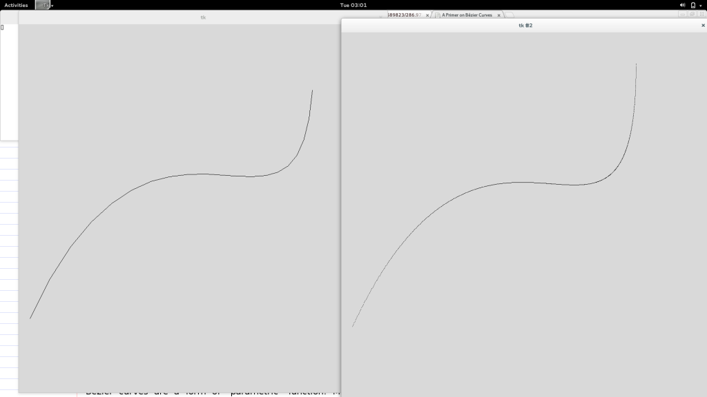
Both splines are exactly the same. On the left is the curve approximated by lines (fast) and on the right drawn with De Casteljau's algorithm (slow).

Conclusion

We saw some performance boosting techniques. From initial 7,3 seconds with De Casteljaus algorithm (plotting 500 quadratic splines) , we made it down to 0.252 seconds! That's around 40 times faster. Of course we could be better, but let's stop here!

Drawing Lines

That's almost it! We also need a algorithm for plotting staright lines. Maybe you think that's a trivial task, but not so fast my dear. There's actually quite a bit of math behind simple even lines! I adopted the algorithm from this site, which offers also a 100 page strong essay about plotting geometrical primitives. The text is quite hard to understand if you don't possess profound mathematical knowledge, but it's still worth a glimpse!

However, this is the line plotting algorithm:

# Yet another implementation taken from
# http://members.chello.at/easyfilter/bresenham.html
# This alogrithm is capable to plot all possible lines in a 2d plane.
def line(self, points):
    if len(points) != 2 or not isinstance(points[1], tuple):
        raise InvalidInputError('To draw a line we need a list of two tuples containing two ints')

    (x0, y0), (x1, y1) = points

    dx = abs(x1-x0)
    dy = -abs(y1-y0)
    sx = [-1, 1][x0= dy):
            err += dy
            x0 += sx     
        if (e2 <= dx):
            err += dx
            y0 += sy

I have shown you some rasterization algorithms and now I am ready to use them to draw my font. In the next article, I will use this code! So stay tuned and send me a letter for Christmas! s!