Introduction to machine learning
This is the beginning of a blog post series that dives into the art of machine learning.
In the past months, I worked a lot with data and I learned that I need to understand the algorithms and problem solving strategies that modern machine learning brings along. To teach myself those concepts, I will create a series of blog posts that cover the fundamentals and some advanced algorithms in machine learning.
The general approach of this blog post series is breadth fist, with the occasional in depth analysis of a interesting algorithm. I try to intuitively understand some concepts, but I will select a few explanatory problems to introduce algorithms and code.
This is the first blog post of this series and will cover a introduction into machine learning as well as the statistical basics of machine learning. I will mostly work with Python3 and the Anaconda Python distribution, since I am familiar with those tools.
This introduction will cover the following topics:
- Some relevant stuff from probability theory and statistics as mathematical background
- Basic algorithms in machine learning such as Bayes and K-Means algorithm
Typical problems that machine learning aims to solve
- machine learning is heavily used in search engine ranking. Algorithms learn based on a wide range of parameters which search results are requested most likely by what kind of user
- Translation of texts within two languages. One approach in translating any text to another text would be to crawl all pages that have mulitlangual support and learn how to translate any text based on this sample set.
- Another example would be classification of faces in images to a label such as the persons name. This is what facebook and instagram do with the images the user uploaded.
- Further well known examples are speech recognition or writing recognition. The aim in those tasks is to translate audio recordings to text and to translate images of handwriting to text.
A special problem that is of major interest for me is the following:
I want to recognize news articles soley based on one input: A link to the document. The algorithm should automatically recognize whether the link shows to a news article and should be able to identify the relvant pieces of information which constitutes a news article:
- An heading
- A publication date
- Optionally a author name
- Optionally a short description
- The article itself
Problem Sets
A problem falls within Binary Classification when our algorithm needs to make a statement whether a value falls in class zero or class one. For example when our machine learning algorithm makes a statement whether a credit card purchase is fraudulent or not, it makes a binary classification.
Multiclass Classification is the extension of Binary Classification. The goal random variable $y \in {1, ..., n}$ can now assume a range of different values. For example we want to classify patient data sets into different levels of health risk based on a range of input factors (very healthy, healthy, ill, terminally ill).
Regression estimates for example the value of a stock in the future or the yield of a business based on past income data or any data point which follows a asummed regression function.
Novelty Detection is a set of problems that search for a metric to detect novel data based on known data from the past.
Some probability theory
I assume that the reader has general knowledge of what a random variable is (for example a dice roll).
A random variable in general maps an event to an result (for example a number). For example a coin toss takes two different outcomes, heads and numbers. Thus this random variable $X$ maps the coin toss into the set ${heads, numbers}$.
A random variable can be discrete (coin toss, two outcomes) or continuous (height of person, indefinitely many measurements).
Another important concept is this of distributions. The probability density function (PDF) always integrates to one.
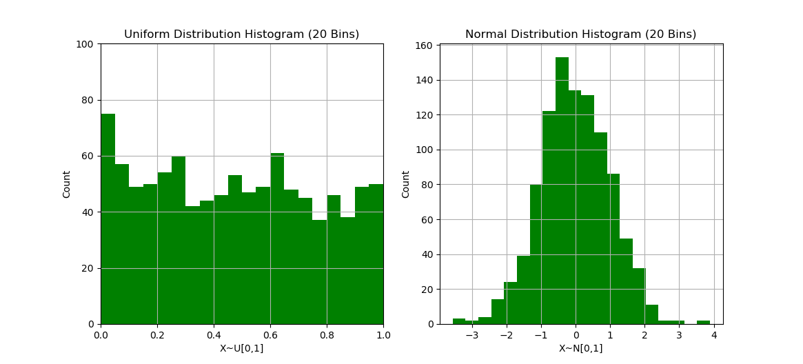
For example two very important and well known distributions are the uniform distribution and the normal distribution. The uniform distribution has the same probability for each $x$ to appear in a interval $[a,b]$. The formula for the uniform distribution is: $$ U(X=x)= \begin{cases} \frac{1}{b-a}, \text{if} x \in [a,b]\ 0, \text{otherwise}\ \end{cases} $$
and the formula for the normal or Gaussian distribution is:
$$ N(X=x)= \frac{1}{\sqrt{2\pi\sigma^2}}\exp{\big(-\frac{(x-\mu)^2}{2\sigma^2}\big)} $$
where $\sigma$ is the variance and $\mu$ is the center/mean of the distribution.
An important concept is also to compute the cumulative distribution function (CDF) $F$ for probability distributions. In general, we integrate over an interval $[a,b]$ to be able to make range queries on the CDF:
$$ P(a \leq X \leq b) = \int_a^b P(X=x) = F(b) - F(a) $$
The mean or expected value of a random variable for example of throwing a dice is $(1+2+3+4+5+6)/6=3.5$.
Then there are measurements of deviance for random variables. The variance of a random variable is the mean of the squared difference from realisation of the random variable and the mean of the random variable. Therefore the variance of the dice example from above is $$ Var(X) = ((1-3.5)^2 + (2-3.5)^2 + (3-3.5)^2 + (4-3.5)^2 + (5-3.5)^2 + (6-3.5)^2)/6 \approx 2.9 $$
This statistical function gives us a quantity of how much the random variable varies around the mean of the distribution. The standard deviation is the square root of the variance.
When we look at two random variables $X$ and $Y$ we can speak of dependent and independent random variables. Two random variables are independent when $$P(X=x, Y=y)=P(x)P(y)$$ if this is not the case they are said to be dependent. Height and weight are usually dependent random variables. Gender and height are also dependent random variables. Hair color and height are however independent from each other.
We speak of independent and identical distributed random variables when a series of random variables $(X_n)_{n \in \mathbb{N}}$ are all independent to each other and they all have the same probability distribution.
When we know that two random variables are dependent on each other, we are interested in the conditional probability. For example what is the conditional probability that a person has a height of 188cm when we know that this person weighs 70kg $P(Height=1.88m, Weight=70kg)$? This conditional probability is most likely lower than the conditional probability $P(Height=1.88m, Weight=80kg)$.
Conditional probability can be formally written as $P(x|y) = \frac{p(x,y)}{p(y)}$
Bayes Theorem
Let $X$ and $Y$ be random variables. Then the following equation is known as Bayes Theorem:
$$ p(y|x)=\frac{p(x|y)p(y)}{p(x)} $$
this follows from the following equality:
$$ p(x,y) = p(x|y)p(y) = p(y|x)p(x) $$
Example for Bayes Theorem
Because Bayes theorem is of such importance, it makes sense to introduce an example in order to get an inuitive understanding of the theorem.
Let's suppose we have a medical test that enables us to test whether a patient has yellow fewer. When a patient is infected with yellow fewer, the test yields always a postive result. On the other hand, the test has for healthy patients a error rate of 2%. Let X be the random variable that tracks the health status of the patient and let T be the random variable that shows the test result of the test. So far we know that $P(T=\text{positive}|X=\text{healthy})=0.02$ and $P(T=\text{negative}|X=\text{healthy})=0.98$.
Let's assume that $0.05%$ of the whole population is infected with yellow fewer in a country like Colombia. We are interested in the probability that the patient is infected with yellow fewer under the condition that the test is positive. Formally we are looking for the solution of $$ p(X=\text{infected}|T=\text{positive}) = \frac{p(T=\text{positive}|X=\text{infected})p(X=\text{infected})}{p(T=\text{positive})} $$
The only term in the equation we don't know is $p(T=\text{positive})$. We can compute it by summing over all possible cases: $$ p(T=\text{positive}) = p(T=\text{positive}, X=\text{infected}) + p(T=\text{positive}, X=\text{healthy}) =\ p(T=\text{positive}|X=\text{infected})p(X=\text{infected}) + p(T=\text{positive}|X=\text{healthy})p(X=\text{healthy}) =\ 1.0\cdot0.0005 + 0.002 \cdot 0.9995 =\ 0.0025 $$
We can now compute the probablity as $p(X=\text{infected}|T=\text{positive})= \frac{1.0 \cdot 0.0005}{0.0025} = 0.2$.
This result is quite astonishing. Even though the test has only a 2% error rate, the test has only a probability of 20% to be corret in confirming an infection if the patient is infected.
So how can we improve the diagnosis and make the test better?
We could introduce more information into account, such as the age or gender of the person to be tested. For example if we fix the age at 22 years, then $p(X=\text{infected}|Age=\text{22}) = 0.001%$ is much lower than the probability that a person of any age is infected (0.05%).
This combination of evidence is a very powerful approach.
We could also repeat measurements with two independent tests $T_1$ and $T_2$ and then the conditional probability from above will be much higher then before:
$$ p(X=\text{infected}|T_1=\text{positive},T_2=\text{positive}) $$
Basic Algorithms
A very good overview of basic machine learning algorithms classified by problem domain can be found here.